Mutation Sequences along Weaves and Amalgamation of Braid Varieties

Yuma Mizuno

This site is a companion to the paper above. Interactive examples show the quiver and coordinate changes at each step of a mutation sequence along a weave. Further diagrams illustrate the decomposition of flag configurations and the relation with tetrahedra.

\operatorname{Conf}(p,q)_{u,v}\ \cong\ \operatorname{Conf}(u,v)\times X(p)\times X(q^{\mathrm{op}})

$\operatorname{Conf}(p,q)$ is the space of pairs of flag sequences following the braids p and q, with prescribed decorations, modulo simultaneous change of frame. The subscripts $u,v$ specify the relative positions of the endpoints of each sequence; here $u=\operatorname{dem}(p),\ v=\operatorname{dem}(q)$ . $\operatorname{Conf}(u,v)$ is the configuration space for reduced words and is isomorphic to a double Bruhat cell. $X(p)$ and $X(q^{\mathrm{op}})$ are braid varieties: spaces of flag sequences with fixed endpoints.

The main theorem describes the compatibility of this decomposition with the cluster structures.

The product decomposition Go straight to the five-step example

THE GEOMETRY

The global product decomposition

Flags and steps of a fixed color

A complete flag in an N-dimensional vector space is a nested sequence of subspaces, one in each dimension.

0\subset F^1\subset F^2\subset\cdots\subset F^N=\mathbb C^N,\quad\dim F^i=i

In type A, a step of color i changes only the i-dimensional subspace. A word such as 1122112 tells us which subspace changes at each step. The flags themselves vary, producing an algebraic variety.

Before a color-1 step

\langle e_1\rangle\subset\langle e_1,e_2\rangle\subset\mathbb C^3

After: the plane stays fixed

\langle e_1+e_2\rangle\subset\langle e_1,e_2\rangle\subset\mathbb C^3

A decorated flag retains extra normalization data: for SLₙ, compatible nonzero volume elements on its subspaces. Keeping these decorations matters for the actual coordinate functions.

$\operatorname{Conf}(p,q)$

B⁰p₁B¹···Bᵐ

⋔opposite at both ends⋔

B₀q₁B₁···Bₙ

Two flag sequences, plus an initial plus decoration and a terminal minus decoration, modulo a simultaneous change of frame by G.

The open endpoint stratum

\operatorname{pos}(B^0,B^m)=u,\qquad\operatorname{pos}(B_0,B_n)=v

u = dem(p) and v = dem(q) are the maximal relative positions allowed by the words. The Demazure product uses braid relations and the rule ii → i.

The three factors and their projection maps

\operatorname{red}:\operatorname{Conf}(p,q)_{u,v}\longrightarrow\operatorname{Conf}(u,v)

Keep the endpoint flags and the two decorations. Replace each long sequence by the unique sequence of the chosen reduced word joining the same endpoints. This factor is isomorphic to the double Bruhat cell Gᵘ,ᵛ.

G^{u,v}=B_+\dot uB_+\cap B_-\dot vB_-

Together these maps form a global isomorphism. Conversely, the reduced configuration supplies the endpoint frames into which the two normalized long sequences are inserted. The original configuration is recovered. Theorem 3.10 ↗

Compatibility with the cluster structure

The sweep constructs a seed in the cluster structure on Conf(p,q) whose coordinates describe this geometric splitting.

CONSTRUCT THE SEED · TYPE A₂

A five-mutation sweep in type A₂

Take p = 1122112 and an empty minus word. Its Demazure product is w₀ = 212. A weave reduces the seven-letter word to this three-letter reduced word through four contractions and one braid move.

\operatorname{Conf}(1122112,\varnothing)_{w_0,e}\cong\operatorname{Conf}(212,\varnothing)\times X(1122112)

The nine initial coordinates

Put a marker at positions 1,2,5,6 on the color-1 string and at positions 3,4,7 on the color-2 string. Consecutive markers delimit a coordinate. Include the unbounded string at each end: five x-variables and four y-variables.

Color 1

x_0=A_{1,[0,1]}

x_1=A_{1,[1,2]}

x_2=A_{1,[2,5]}

x_3=A_{1,[5,6]}

x_4=A_{1,[6,\infty]}

Color 2

y_0=A_{2,[0,3]}

y_1=A_{2,[3,4]}

y_2=A_{2,[4,7]}

y_3=A_{2,[7,\infty]}

These are actual generalized minors. For this SL₃ example, define the matrices:

B_1(z)=\begin{pmatrix}z&-1&0\\1&0&0\\0&0&1\end{pmatrix}

B_2(z)=\begin{pmatrix}1&0&0\\0&z&-1\\0&1&0\end{pmatrix}

g_r=B_{\beta_1}(z_1)\cdots B_{\beta_r}(z_r),\qquad t_i=\omega_i(h)

A_{i,[r,s]}=t_i\Delta_{\omega_i}(g_r)

For SL₃, Δω₁ is the top-left entry and Δω₂ is the top-left 2 × 2 minor. These functions and the exchange matrix specify the initial seed.

WEAVE

Letters remaining：7Retained coordinates：0

Start with the Shen–Weng seed of the seven-letter word. The five bounded internal strings are mutable; the four boundary strings are frozen.

Coordinate change

\Sigma_0=(x_1,x_2,x_3,y_1,y_2;\ x_0,x_4,y_0,y_3)

Notation: aᵢ = Aσᵢ in the manuscript; b is the coordinate A′₂,[1,2] created by the braid move.

QUIVER

○ mutable□ frozen◌ next mutation⇢ weight ½

Select a vertex in the quiver to inspect it.

Inspect the exact exchange matrix

εᵢⱼ > 0 means i → j. All nine rows are included, also the frozen–frozen entries.
ε	$x_0$	$x_1$	$x_2$	$x_3$	$x_4$	$y_0$	$y_1$	$y_2$	$y_3$
$x_0$	·	-1	·	·	·	½	·	·	·
$x_1$	1	·	-1	·	·	·	·	·	·
$x_2$	·	1	·	-1	·	-1	·	1	·
$x_3$	·	·	1	·	-1	·	·	·	·
$x_4$	·	·	·	1	·	·	·	-1	½
$y_0$	−½	·	1	·	·	·	-1	·	·
$y_1$	·	·	·	·	·	1	·	-1	·
$y_2$	·	·	-1	·	1	·	1	·	-1
$y_3$	·	·	·	·	−½	·	·	1	·

The sweep seed in the Shen–Weng cluster structure

Every step is a mutation of the original Shen–Weng seed. This proves that the final coordinates belong to the existing cluster structure. The remaining task is to identify the final quiver and its geometric coordinate functions.

BOUNDARY WEIGHTS

Boundary cycles and frozen amalgamation

A Lusztig cycle on the weave determines the mixed arrows at its quiver vertex. Choose γᵢ to follow its path on the left and see the corresponding part of the full quiver at aᵢ on the right.

Choose a cycle

Cycle on the weave

\gamma_2

\partial\gamma_2=(1,0,0)

Terminal weights and quiver arrows

a_2

y_0\longrightarrow a_2\longrightarrow b

cycle weight / mixed arrowarrow already in the terminal quiver○ mutable　□ frozen

Weight 1 at the first 2 of 212 gives y₀ → a2 → b. The existing arrow b → y₀ closes the triangle. The two different cycles γ₂ and γ₃ reach this same terminal letter.

Transport rules and incidence entries

Transport the cycle weights

At its own trivalent vertex σᵢ, γᵢ starts with weight 1 on the outgoing edge and 0 above. Later contractions and the braid move use:

ii → i

(r,s)\longmapsto\min(r,s)

121 → 212

(r,s,t)\longmapsto(s+t-m,m,r+s-m)

m=\min(r,t)

Signed incidence at the terminal word

At each letter, take the left string minus the right string.

(w_1,w_2,w_3)\mapsto w_1(e_{y_0}-e_b)+w_2(e_{x_0}-e_{x_4})+w_3(e_b-e_{y_3})

$\varepsilon_{\ell,a_1}>0\iff\ell\longrightarrow a_1$
ℓ	$\varepsilon_{\ell,a_1}$	Arrow
$x_0$	0	$\text{—}$
$b$	0	$\text{—}$
$x_4$	0	$\text{—}$
$y_0$	0	$\text{—}$
$y_3$	0	$\text{—}$

$\varepsilon_{\ell,a_2}>0\iff\ell\longrightarrow a_2$
ℓ	$\varepsilon_{\ell,a_2}$	Arrow
$x_0$	0	$\text{—}$
$b$	-1	$a_2\longrightarrow b$
$x_4$	0	$\text{—}$
$y_0$	1	$y_0\longrightarrow a_2$
$y_3$	0	$\text{—}$

$\varepsilon_{\ell,a_3}>0\iff\ell\longrightarrow a_3$
ℓ	$\varepsilon_{\ell,a_3}$	Arrow
$x_0$	0	$\text{—}$
$b$	-1	$a_3\longrightarrow b$
$x_4$	0	$\text{—}$
$y_0$	1	$y_0\longrightarrow a_3$
$y_3$	0	$\text{—}$

$\varepsilon_{\ell,a_4}>0\iff\ell\longrightarrow a_4$
ℓ	$\varepsilon_{\ell,a_4}$	Arrow
$x_0$	0	$\text{—}$
$b$	1	$b\longrightarrow a_4$
$x_4$	0	$\text{—}$
$y_0$	0	$\text{—}$
$y_3$	-1	$a_4\longrightarrow y_3$

\mathcal D(\mathfrak W)=\{\sigma:\partial\gamma_\sigma\ne0\}=\{\sigma_2,\sigma_3,\sigma_4\}

Consequently the endpoint stratum is exactly {a₂a₃a₄ ≠ 0}. The variables a₁ and b may vanish there; the stratum is larger than this one seed torus. Theorem 5.22 ↗

Amalgamation along the boundary vertices

Extended terminal quiver

Q^{\mathrm{ext}}(212;\mathfrak W)

5 + 3

Five strings, plus one frozen copy of each boundary cycle.

∗a₂,a₃,a₄

Weave quiver

Q(\mathfrak W)

The four contraction vertices; a₂, a₃, a₄ are frozen.

=8 + 4 − 3

Amalgamated quiver

Q^{\mathrm{am,fr}}(\mathfrak W)

Identify the shared frozen copies and add their exchange entries.

Cancellation of the frozen boundary terms

\underbrace{(I_{\sigma\tau}-\Omega_{\sigma\tau})}_{Q(\mathfrak W)}+\underbrace{\Omega_{\sigma\tau}}_{Q^{\mathrm{ext}}}=I_{\sigma\tau}

The weave quiver includes a boundary correction to the local intersection pairing I. The extension adds the opposite correction Ω. Their sum is the contraction block of the sweep quiver, including entries between frozen vertices.

Q^{\mathrm{sweep}}(\mathfrak W)=\operatorname{defrost}_{\mathcal D(\mathfrak W)}Q^{\mathrm{am,fr}}(\mathfrak W)

The sweep theorem identifies the full quiver before localization. Freezing the boundary set recovers the amalgamation above. Theorem 4.27 ↗

COORDINATE FUNCTIONS

Cartan monomials and product coordinates

The boundary decoration determines how the sweep coordinates relate to the coordinates on the three product factors. Cartan monomials express this dependence.

A_\ell^{\mathrm{am}}=A_\ell^\delta\,M_\ell,\qquad A_\sigma^{\mathrm{am}}=A_\sigma^{\mathfrak W}

Braid-variety coordinates agree exactly. Terminal coordinates are multiplied by Laurent monomials in the boundary variables.

Boundary weights determine the monomials

The cycles for a₂ and a₃ have weight at the first letter of 212; the cycle for a₄ has weight at the third letter. Collect the weights at each letter as a monomial:

u_t=\prod_{\sigma\in\mathcal D(\mathfrak W)}a_\sigma^{\partial\gamma_\sigma(t)},\qquad(u_1,u_2,u_3)=(a_2a_3,1,a_4)

Transport these Cartan factors along 212 and evaluate the fundamental weights. This gives the five corrections in the table, expressed as identities of coordinate functions.

The five strings of the terminal word 212
String	Product coordinate	Cartan monomial	Sweep coordinate
$(2,[0,1])$	$r_0$	$1$	$y_0=r_0$
$(1,[0,2])$	$s_0$	$1$	$x_0=s_0$
$(2,[1,3])$	$r_1$	$a_2a_3$	$b=r_1a_2a_3$
$(1,[2,\infty])$	$s_1$	$a_2a_3$	$x_4=s_1a_2a_3$
$(2,[3,\infty])$	$r_2$	$a_4$	$y_3=r_2a_4$

Cartan propagation and the exponent formula

First package terminal weights as uₜ = ∏ aσ^(∂γσ(t)). Propagate the Cartan factor through the terminal word. At a plus letter i, the coroot degree transforms by Hₜ = sᵢHₜ₋₁ + λ(t)αᵢ∨; minus letters use the reverse recursion. Evaluate fundamental weights on the resulting degrees to get cℓ(λ).

M_\ell=\prod_{\sigma\in\mathcal D(\mathfrak W)}a_\sigma^{c_\ell(\partial\gamma_\sigma)}

For this SL₃ example the Cartan factors are:

h_0^+=1,\quad h_1^+=\operatorname{diag}(1,u_1,u_1^{-1}),\quad h_2^+=\operatorname{diag}(u_1,1,u_1^{-1})

h_3^+=\operatorname{diag}(u_1,u_3/u_1,u_3^{-1})

Their fundamental-weight evaluations give (1,1,a₂a₃,a₂a₃,a₄), exactly the table above. §5.1 example ↗

The coordinates on each product factor

(r_0,s_0,r_1,s_1,r_2)=\left(y_0,x_0,\frac b{a_2a_3},\frac{x_4}{a_2a_3},\frac{y_3}{a_4}\right)

The boundary variables a₂, a₃, a₄ are invertible on the endpoint stratum, so division by the corrections is defined there. The first factor has one mutable variable r₁. The braid factor has one mutable variable a₁ and frozen variables a₂, a₃, a₄. These are the two mutable variables of the localized seed, expressed in product coordinates.

Preservation of the exchange ratios

Corresponding mutable A-coordinates may differ by frozen Laurent monomials. The exchange ratios Xⱼ = ∏ Aᵢ^εⱼᵢ agree exactly. In this example:

X_b=\frac{x_4y_0a_4}{x_0y_3a_2a_3}=\frac{s_1r_0}{s_0r_2}=X_{r_1}

X_{a_1}=\frac{a_3}{a_4}

The boundary factors cancel in the first ratio. The braid ratio already depends only on its own factor. Theorem 5.23 ↗

THE GENERAL RESULT

Cluster localization and the product isomorphism

Let G be a connected, simply connected semisimple complex algebraic group of finite type. For any positive braids p,q with Demazure products u,v, choose a double Demazure weave ending at reduced words for u and v.

Start with the existing seed

A double word β combines the plus word p and the minus word q. Use its Shen–Weng seed.

Sweep from top to bottom

Use the rank-two mutation sequence for each braid move. At each contraction ii → i, mutate the middle string and retain that vertex.

Read and freeze the boundary

Transport each based Lusztig cycle. Freeze precisely D(W), the vertices whose terminal weights are nonzero.

Divide out the Cartan corrections

The monomial factors Mℓ convert terminal coordinates to product coordinates. The braid coordinates agree directly and the exchange ratios are preserved.

MAIN THEOREM · THEOREM 1.1

Cluster localization of the endpoint stratum

\operatorname{Conf}(p,q)_{u,v}=\bigcap_{\sigma\in\mathcal D(\mathfrak W)}\{A_\sigma^{\mathrm{sweep}}\ne0\}

\mathcal A(\Sigma^{\mathrm{fr}})=\mathcal U(\Sigma^{\mathrm{fr}})=\mathcal A(\Sigma)[(A_\sigma)^{-1}\mid\sigma\in\mathcal D(\mathfrak W)]

\mathcal A(\Sigma^{\mathrm{fr}})\cong\mathcal O\bigl(\operatorname{Conf}(p,q)_{u,v}\bigr)

Here Σ is the sweep seed, Σᶠʳ is obtained by freezing D(W), A is the cluster algebra, and U is the upper cluster algebra. Freezing is a combinatorial operation; the theorem proves that it really gives the coordinate ring of the specified geometric open set.

The splitting as a quasi-cluster isomorphism

\operatorname{split}:\operatorname{Conf}(p,q)_{u,v}\xrightarrow{\sim}\operatorname{Conf}(u,v)\times X(p)\times X(q^{\mathrm{op}})

This is a quasi-cluster isomorphism. Moreover, cluster variables on either braid-variety factor pull back to actual cluster variables of the localized seed.

Read the full statement ↗

Proof structure: geometry, quivers, functions, localization

Geometry · §3

Bruhat factorization normalizes the long flag sequences. Reduction and insertion give mutually inverse maps for the global product decomposition.

Quivers · §4

Induct over elementary weave moves, tracking word vertices, retained vertices, mixed arrows and the full frozen block. Boundary corrections cancel to give the terminal amalgamation.

Functions · §5.1–5.3

Use generalized-minor identities, flag propagation and Cartan homogeneity to match each mutation with the actual geometric coordinate transformation. Iterating gives the amalgamated coordinate formula.

Localization · §5.4

Express the endpoint minors as monomials in the boundary coordinates, identify the open set, then compare with the independently known coordinate rings of the three product factors.

SPLICING

Half-twist extensions and splicing

Forget one decoration. If Δ is a reduced positive braid for w₀ and dem(p) = w₀, the half-decorated splitting gives:

X(p)\times X(\Delta\Delta)\xrightarrow[\text{quasi-cluster}]{\sim}\mathcal U_{r,w_0}(p\Delta)\subset X(p\Delta)

Here r is the length of p. There is also a corresponding map into X(Δp), with X(ΔΔ) as the first factor. This proves the GKSS conjecture for these half-twist extension cases.

The target is the splicing open subset shown above; its seed comes from the same sweep and freezing construction.

Corollary 1.3 and §6 ↗

TETRAHEDRAL FLIPS

Tetrahedral projection and sweep mutations

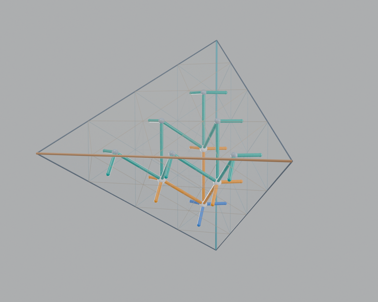
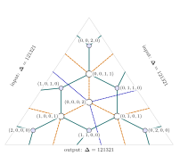
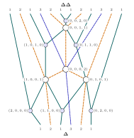
\boldsymbol\Delta=(1)(21)\cdots((N-1)\cdots1),\qquad\mathfrak W:\boldsymbol\Delta\boldsymbol\Delta\longrightarrow\boldsymbol\Delta

In type A of rank N − 1, the N-decomposition of a tetrahedron has octahedra indexed by nonnegative tuples (a,b,c,d) with a+b+c+d=N−2. Project from one vertex onto the opposite face. Each octahedron becomes a vertex of the weave, and neighboring octahedra are joined by its strands.

Tetrahedral projection of the A₃ weave, with vertices labeled by (a,b,c,d). — Tetrahedral projection

The string diagram of the same A₃ weave from ΔΔ to Δ, with the corresponding vertex labels. — String diagram

Figure 3 in the manuscript ↗

The layer d determines the local move

$d=0:\quad11\longrightarrow1$
The outer layer projects to trivalent contractions of color 1. Each contraction contributes one mutation.

$d>0:\quad d\,(d+1)\,d\longleftrightarrow(d+1)\,d\,(d+1)$
The other layers project to six-valent braid vertices of colors d and d+1. Each type A₂ braid move also contributes one mutation. Commutations contribute none.

N = 4: Δ = 121321; the three layers of the tetrahedron
Layer	Weave vertex	Mutations
$d=0$	Color-1 contraction	6
$d=1$	$121\leftrightarrow212$	3
$d=2$	$232\leftrightarrow323$	1

Ptolemy relations as exchange relations

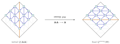
At each corresponding vertex, the sweep exchange relation is the Ptolemy relation of that octahedron. The complete sweep therefore realizes the tetrahedral flip. Counting the tuples in each layer gives:

\#\{(a,b,c)\in\mathbb Z_{\ge0}^3:a+b+c=N-2-d\}=\binom{N-d}{2}

The outer layer contributes the contractions; summing over the remaining layers gives the braid mutations.

\underbrace{\binom N2}_{\text{contractions}}+\underbrace{\binom N3}_{\text{braid moves}}=\binom{N+1}3,\qquad N=4:\quad6+(3+1)=10

The initial quiver for ΔΔ and the final sweep quiver, joined by the sweep mutation sequence. — The quivers before and after the sweep. Figure 4 ↗

The manuscript also gives a C₃ weave as an example beyond type A. Projection, weave and sweep quivers: §1.4 ↗

Read the paper